Data Structures. Graph

18 декабря 2023 г.

This is a short expanded summary of the section on graphs in the book Computer Science Guide by William Springer.

The Königsberg Bridge Problem

The Königsberg bridge problem is where graph theory began.

Problem: In the city of Königsberg (now Kaliningrad), a river splits the city into four parts connected by seven bridges. The question was: is it possible to walk through the city crossing each bridge exactly once?

Leonhard Euler was asked this question. His key insight was that topological deformations do not matter (changing size or shape does not affect the problem as long as connections remain the same). He called this the geometry of position.

We can simplify the map by replacing each land area with a vertex and each bridge with an edge connecting vertices. This produces a graph.

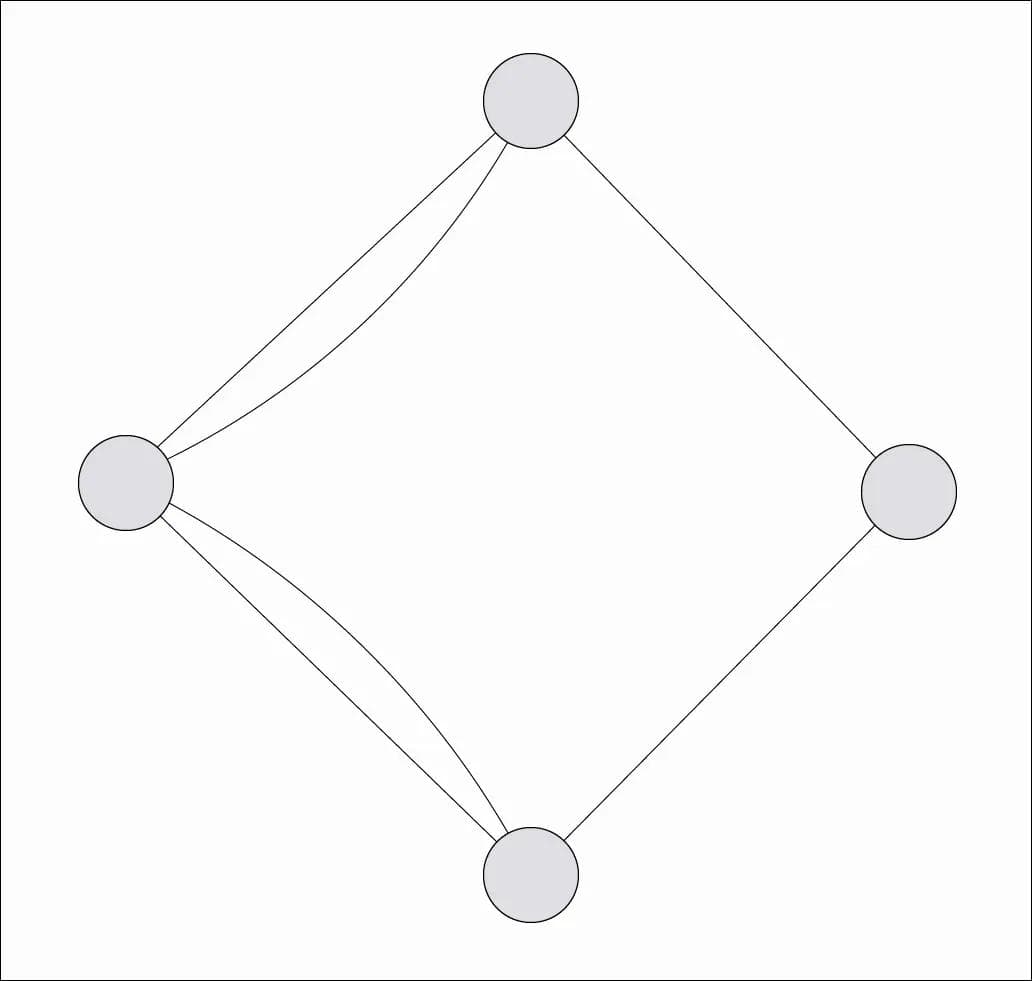
Graph based on the Königsberg bridge problem

The key logical conclusion: to enter land and then leave it, two different bridges are required.

Any land area (except the start and end point of the route) must have an even number of bridges connected to it.

In Königsberg, each of the four land areas had an odd number of bridges, making the problem unsolvable.

An Eulerian path is a path through a graph that visits every edge exactly once.

Some problems are NP-hard on general graphs but have efficient (often O(n)) solutions on graphs with specific properties.

Basic Information

A graph is a way of representing relationships within a set of data. Graphs are commonly visualized as circles (vertices) connected by lines (edges).

Adjacent vertices are connected by an edge, while non-adjacent vertices are not.

A vertex is also called a node. The two terms are often used interchangeably, although there are exceptions. For example, a point in a polygon where two or more edges meet is always called a vertex. A memory structure that stores a vertex together with its set of edges is typically called a node.

A subgraph of a graph consists of any subset of the graph's vertices together with any subset of the edges (that also belong to the original graph) connecting those vertices.

An induced subgraph consists of a subset of vertices together with all edges from the original graph that connect those vertices.

A proper subset contains fewer vertices than the original graph.

A non-proper subset (or simply subset) may contain all the vertices of the original graph.

A graph class is a (typically infinite) collection of graphs that share a particular property. Whether a graph belongs to a given class depends on whether it satisfies that property.

A bipartite graph is a graph whose vertices can be divided into two disjoint sets such that every edge connects a vertex from one set to a vertex in the other.

Bipartite graphs are used in coding theory (which includes cryptography, data compression, and error correction), Petri nets (used for modeling system behavior), social network analysis, and cloud computing.

A complete graph (or clique, when referring to a complete subgraph) is a graph that contains every possible edge between its vertices.

Example: K₈ is a complete graph with eight vertices.

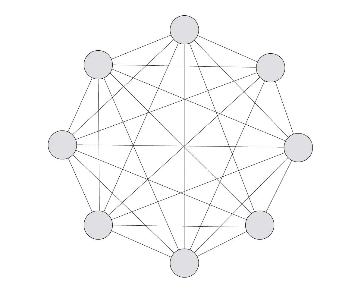
The letter K with an integer subscript denotes a complete graph with the corresponding number of vertices.

An independent set (or internally stable set) is a set of vertices with no edges between them.

A connected graph/subgraph is a graph in which there exists a path from any vertex to any other vertex.

A disconnected graph consists of several connected components.

Example: A disconnected graph with six connected components, each of size 1.

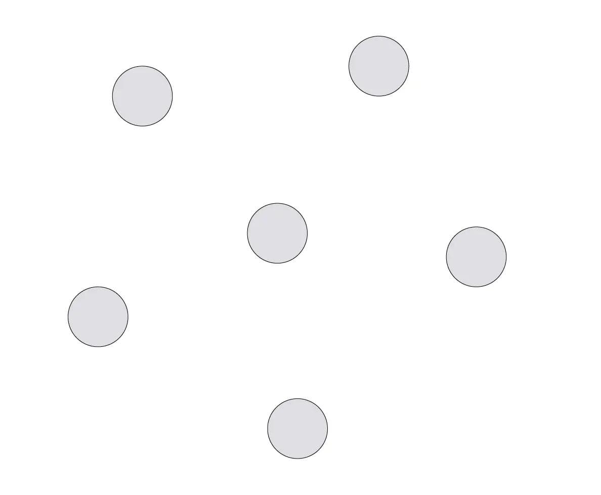
When we say "graph" without specifying otherwise, we always mean a simple graph.

A non-simple graph is a graph that contains loops (an edge that starts and ends at the same vertex).

A multigraph is a graph that contains multiple edges (several edges connecting the same pair of vertices).

Directed and Undirected Graphs

An undirected graph (a simple graph) is a graph where edges can be traversed in both directions.
If A is connected to B, then B is also connected to A.

A directed graph (or digraph) is a graph where each edge has a direction.
For example, if Albert sends a message to Victor, this does not mean that Victor will always reply to Albert. The edge from A to B only indicates the direction of the message. If Victor replies, there will be another edge directed in the opposite direction, from B to A.

A symmetric directed graph is a graph where for every directed edge there exists another edge connecting the same two vertices but directed in the opposite direction. It is equivalent to an undirected graph with one edge between each pair of connected vertices. Therefore, ordinary (undirected) graphs can be considered a special case of directed graphs.

A directed (antisymmetric) graph is a graph where between any two vertices there can exist only one directed edge (in one direction only).

Cyclic and Acyclic Graphs

A cyclic graph is a graph that contains at least one cycle.

A cycle is a path that starts and ends at the same vertex.
Every complete graph is cyclic.
If the graph is directed, all edges in the cycle must have the same direction.

An acyclic graph is a graph with no cycles. In such a graph, there is at most one path between any two vertices.

Weighted and Unweighted Graphs

In reality, not all edges in a graph have the same length.

An unweighted graph is a graph where edges only indicate which vertices are directly connected.

A weighted graph is a graph where each edge has an assigned weight. These are often non-negative integers. The weight represents the cost of using an edge.

The meaning of a weight depends on what the graph represents.

For a weighted graph, it is necessary to store not only the fact that two vertices are connected but also the weight of the edge connecting them.

For example, if a subway map is represented as a graph, the time required to travel between stations would be the weight of the edge.

Graph Representation

Graph Size Notation

n — the number of vertices.
m — the number of edges.

Usually, the set of vertices is denoted by the letter V, and the set of edges by the letter E. Therefore:

|V| = n — the size of the vertex set.
|E| = m — the size of the edge set.

The size of the graph is determined by the number of vertices (n) and edges (m).

The amount of memory required to store a graph depends on the representation method used.

Graphs are usually represented as:

Graph Representation Using Adjacency Lists

Each vertex in the graph is stored together with a list of its adjacent vertices.

This representation is efficient for:

Sparse graphs — an adjacency list is more memory-efficient because there is no need to store O(n²) zero values, and all existing edges can be traversed easily.
Dynamic graphs (graphs that change over time) — adding and removing vertices is simpler than with other graph representations.

JavaScript

1// Complete graph
2const fullGraph = {
3	1: [2, 3, 4, 5, 6, 7, 8],
4	2: [1, 3, 4, 5, 6, 7, 8],
5	3: [1, 2, 4, 5, 6, 7, 8],
6	4: [1, 2, 3, 5, 6, 7, 8],
7	5: [1, 2, 3, 4, 6, 7, 8],
8	6: [1, 2, 3, 4, 5, 7, 8],
9	7: [1, 2, 3, 4, 5, 6, 8],
10	8: [1, 2, 3, 4, 5, 6, 7],
11};
12
13// Disconnected graph
14const disconnectedGraph = {
15  1: [],
16  2: [],
17  3: [],
18  4: [],
19  5: [],
20  6: [],
21}

The space complexity is O(n + m).

For a sparse graph (one with relatively few edges), the space complexity is O(n).
For a dense graph (a graph with many edges, such as a complete or nearly complete graph), the space complexity is O(n²), since m = O(n²).

Graph Representation Using an Adjacency Matrix

An adjacency matrix has the following properties:

Each cell of the matrix contains either 0 (the corresponding vertices are not adjacent) or 1 (the vertices are adjacent).
The number of 1s in the matrix is equal to twice the number of edges in the graph (for an undirected graph).
The cells on the main diagonal are always 0, since no vertex has an edge that starts and ends at itself in a simple graph.
An adjacency matrix consists of n rows and n columns, so it requires O(n²) space. For dense graphs, this representation remains space-efficient because the number of edges is also O(n²).

JavaScript

1// Complete graph
2const fullGraph = [
3  [0, 1, 1, 1, 1, 1, 1, 1],
4  [1, 0, 1, 1, 1, 1, 1, 1],
5  [1, 1, 0, 1, 1, 1, 1, 1],
6  [1, 1, 1, 0, 1, 1, 1, 1],
7  [1, 1, 1, 1, 0, 1, 1, 1],
8  [1, 1, 1, 1, 1, 0, 1, 1],
9  [1, 1, 1, 1, 1, 1, 0, 1],
10  [1, 1, 1, 1, 1, 1, 1, 0],
11]
12
13// Disconnected graph
14const disconnectedGraph = [
15  [0, 0, 0, 0, 0, 0,],
16  [0, 0, 0, 0, 0, 0,],
17  [0, 0, 0, 0, 0, 0,],
18  [0, 0, 0, 0, 0, 0,],
19  [0, 0, 0, 0, 0, 0,],
20  [0, 0, 0, 0, 0, 0,],
21]

For a multigraph, some of these properties no longer hold. Matrix entries may be greater than 1 (since multiple edges can connect the same pair of vertices), and the main diagonal may contain non-zero values (because loops can connect a vertex to itself).

This representation is efficient for:

Applications that require predictable performance — an adjacency matrix provides direct access to edges. For example, A[i][j] = 1 indicates that vertices i and j are adjacent. Checking whether an edge exists takes constant time, O(1).
Real-time applications — it is often acceptable to sacrifice some memory efficiency in exchange for guaranteed upper bounds on operation time. Since edge lookups in an adjacency matrix always take constant time, it is well suited for systems with strict timing requirements.

Examples of adjacency list and adjacency matrix representations for directed and undirected graphs can be found here.

Representing a Weighted Graph

As an example of a weighted graph, consider a subway map, where the weight of an edge represents the travel time between stations in minutes.

Adjacency Matrix

Instead of using 0 and 1 to indicate whether two vertices are connected, the edge weight is stored in the corresponding cell of the matrix.

JavaScript

1const Graph = [
2  [0, 10, 8, 0, 0, 0,],
3  [0, 0, 0, 0, 0, 12,],
4  [0, 0, 0, 11, 5, 0,],
5  [0, 0, 0, 0, 0, 10,],
6  [0, 0, 0, 0, 0, 11,],
7]

Adjacency List

For each vertex, store a list of its adjacent vertices together with the weight of each connecting edge.

JavaScript

1// Example of a weighted graph using nested arrays
2let weightedGraph1 = {
3	a: [
4		[b, 10],
5		[c, 8],
6	],
7	b: [[f, 12]],
8	c: [
9		[d, 11],
10		[e, 5],
11	],
12	d: [[f, 10]],
13	e: [[f, 11]],
14};
15
16// Using objects
17let weightedGraph2 = {
18	a: { b: 10, c: 8 },
19	b: { f: 12 },
20	c: { d: 11, e: 5 },
21	d: { f: 10 },
22	e: { f: 11 },
23};

Graph Representation in Memory

In memory, a graph is often stored as a collection of nodes. Each node represents a single vertex and contains a set of references (pointers) to other nodes. Each reference corresponds to an edge leading to another vertex.

Chordless Cycles

A chord is an edge connecting two vertices of a cycle that is not itself part of the cycle.

A chordless cycle (also called an induced cycle) is a cycle consisting of at least four vertices that contains no chords.

Example: A chordless cycle with six vertices.

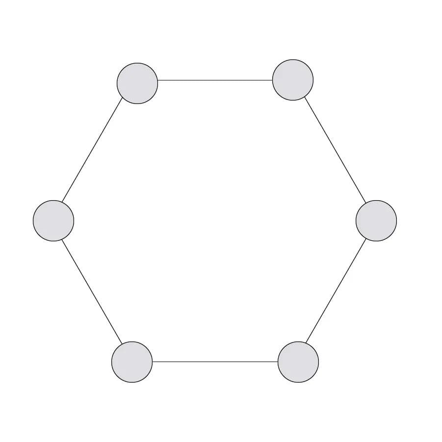
A chordal graph is a graph that contains no induced chordless cycles.

Graph Coloring

Many graph problems involve graph coloring.

Graph coloring is a way of assigning labels (traditionally called colors) to the vertices or edges of a graph. In vertex coloring, the goal is to partition the vertices into independent sets.

A proper vertex coloring is an assignment of colors such that no two adjacent vertices (vertices connected by an edge) have the same color.

A proper edge coloring is an assignment of colors such that no two edges incident to the same vertex share the same color.

Graph coloring does not necessarily use actual colors. For example, Sudoku can be viewed as a graph coloring problem in which the labels are the numbers 1 through 9.

Chromatic Number of a Graph

The chromatic number of a graph is the minimum number of colors required to produce a proper vertex coloring of the graph.

The chromatic number is:

At most 4 for a planar graph (a graph that can be drawn so that no two edges intersect except at their endpoints).
1 for a graph with no edges, since all vertices can be assigned the same color.
n for a complete graph with n vertices, because every pair of vertices is adjacent and therefore each vertex must have a different color.

Time Complexity

Checking whether an arbitrary graph is 2-colorable (bipartite) can be done in linear time. Since only two colors are used, it is sufficient to color adjacent vertices with different colors. The algorithm terminates when either:

all vertices have been successfully colored, or
two adjacent vertices are found to have the same color.

However, determining whether a graph is 3-colorable is an NP-complete problem.

In general, algorithms that determine whether a graph is k-colorable require exponential time.

If the graph belongs to a specific class (for example, a perfect graph), a valid coloring can be found in polynomial time.

Applications

Graph coloring algorithms are commonly used in applications such as:

scheduling,
data analysis,
networking, and more.

For example, consider the problem of scheduling one-hour meetings where different meetings involve different people and require different equipment. Represent each meeting as a vertex, and add an edge between two vertices if the corresponding meetings involve the same person or the same piece of equipment.

Finding a minimum coloring of the graph tells us the minimum number of different time slots required so that no conflicting meetings are scheduled at the same time.

Graph-Based Data Structures

JavaScript Implementation

The following example is taken from this article.

Main Methods

addVertex — adds a new vertex.
addEdge — adds a new edge.

JavaScript

1class Graph {
2	constructor() {
3		this.vertices = {}; // Graph adjacency list
4	}
5
6	addVertex(value) {
7		if (!this.vertices[value]) {
8			this.vertices[value] = [];
9		}
10	}
11
12	addEdge(vertex1, vertex2) {
13		if (!(vertex1 in this.vertices) || !(vertex2 in this.vertices)) {
14			throw new Error("There are no such vertices in the graph.");
15		}
16
17		if (!this.vertices[vertex1].includes(vertex2)) {
18			this.vertices[vertex1].push(vertex2);
19		}
20		if (!this.vertices[vertex2].includes(vertex1)) {
21			this.vertices[vertex2].push(vertex1);
22		}
23	}
24}
25
26const graph = new Graph();
27
28graph.addVertex("A");
29graph.addVertex("B");
30graph.addVertex("C");
31graph.addVertex("D");
32graph.addVertex("E");
33graph.addVertex("F");
34graph.addVertex("G");
35graph.addVertex("H");
36
37graph.addEdge("A", "B");
38graph.addEdge("A", "C");
39graph.addEdge("C", "D");
40graph.addEdge("C", "E");
41graph.addEdge("A", "F");
42graph.addEdge("F", "G");
43
44// Graph {
45//   vertices: {
46//     A: [ 'B', 'C', 'F' ],
47//     B: [ 'A' ],
48//     C: [ 'A', 'D', 'E' ],
49//     D: [ 'C' ],
50//     E: [ 'C' ],
51//     F: [ 'A', 'G' ],
52//     G: [ 'F' ],
53//     H: []
54//   }
55// }